Research Overview
In this ongoing research, we work on the structure-preserving discretization of the incompressible Navier-Stokes (NS) equations
[math] \partial_t v + \omega\times v + \frac{1}{\text{Re}} \text{curl}(\omega)+ \text{grad}(p) = 0 [/math]
[math] \omega = \text{curl}(v) [/math]
[math] 0 = \text{div}(v) [/math]
expressed in the rotational form with [math] v,\omega,p [/math] denoting the velocity vector-field, vorticity pseudo-vector-field, and pressure scalar-field, respectively.
We discretize the PDEs above using the dual-field method proposed in [1] which is based on two representations of the NS equations abvoe that are Hodge-dual to each other. Using scalar-valued forms and Finite-Element Exterior Calculus (FEEC), the two representations of the spatially-discretized dynamics have an algebraic structure of the form:
[math]\begin{pmatrix} M_1 + \frac{\Delta t}{2} S(\tilde{\omega}_{\tilde{k}}) & \frac{\Delta t}{2 \text{Re}} C^\top & \Delta t\ G \\ -C & M_2 & 0\\ -G^\top & 0 &0\\ \end{pmatrix} \begin{pmatrix} v_{k+1} \\ \omega_{k+1} \\ p_{k+1/2}\end{pmatrix} = \begin{pmatrix} M_1 – \frac{\Delta t}{2} S(\tilde{\omega}_{\tilde{k}}) &- \frac{\Delta t}{2 \text{Re}} C^\top & 0 \\ 0 & 0 & 0 \\ 0 & 0 & 0 \\ \end{pmatrix} \begin{pmatrix} v_{k} \\ \omega_{k} \\ p_{k-1/2}\end{pmatrix} [/math]
[math]\begin{pmatrix} \tilde{M}_1 + \frac{\Delta t}{2} \tilde{S}(\omega_k) & \frac{\Delta t}{2 \text{Re}} C & – \Delta t\ D^\top \\ -C^\top & \tilde{M}_2 & 0\\ D & 0 &0\\ \end{pmatrix} \begin{pmatrix} \tilde{v}_{\tilde{k}+1} \\ \tilde{\omega}_{\tilde{k}+1} \\ \tilde{p}_{\tilde{k}+1/2}\end{pmatrix} = \begin{pmatrix} \tilde{M}_1 – \frac{\Delta t}{2} \tilde{S}(\omega_k) &- \frac{\Delta t}{2 \text{Re}} C & 0 \\ 0 & 0 & 0 \\ 0 & 0 & 0 \\ \end{pmatrix} \begin{pmatrix} \tilde{v}_\tilde{k} \\ \tilde{\omega}_\tilde{k} \\ \tilde{p}_{\tilde{k}-1/2}\end{pmatrix} [/math]
where [math] (v_k,\omega_k,p_{k+1/2}) [/math] denote the discrete velocity, vorticity, and pressure variables of the first (primal) formulation, while [math] (\tilde{v}_\tilde{k},\tilde{\omega}_\tilde{k},\tilde{p}_{\tilde{k}+1/2}) [/math] denote the discrete velocity, vorticity, and pressure variables of the second (dual) formulation. The two systems are coupled together via the vorticity variables. By using a staggered temporal scheme, the primal system is solved at half-integer time steps and the dual system at integer time steps (i.e. [math] \tilde{k} = k+1/2 [/math]) and one ends up solving two linear systems sequentially every time-step.
Thanks to the structure-preserving discretization properties of this dual-field discretization scheme, its numerical solution preserves the conserved quantities underlying the PDEs of the NS equations above. Namely, the total kinetic energy, helicity, and mass in the domain are preserved with very high precision that reaches machine-precision when direct solvers are used.
Within this research, I have implemented this solver using Firedrake and Docker and it is available open-source on Gitlab. The solver is currently applicable to periodic spatial domains only. Its extension to include generic boundary conditions is still in progress. Some of the results of benchmark problems in a periodic domain are shown below
Taylor-Green Vortex problem
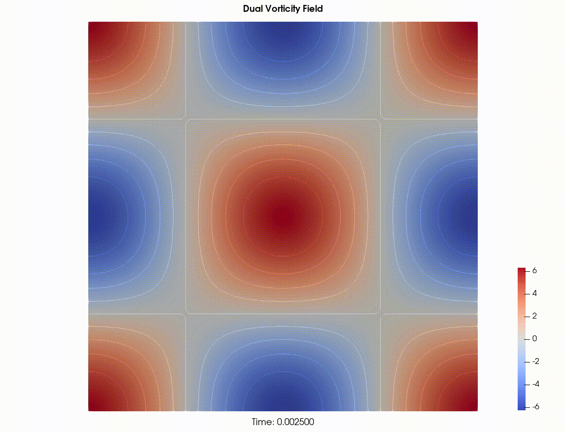
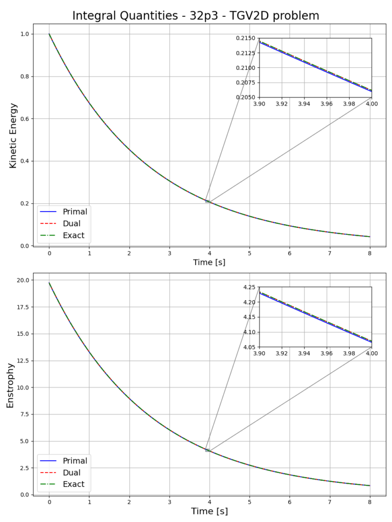
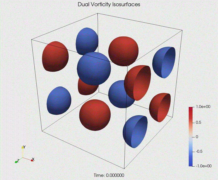
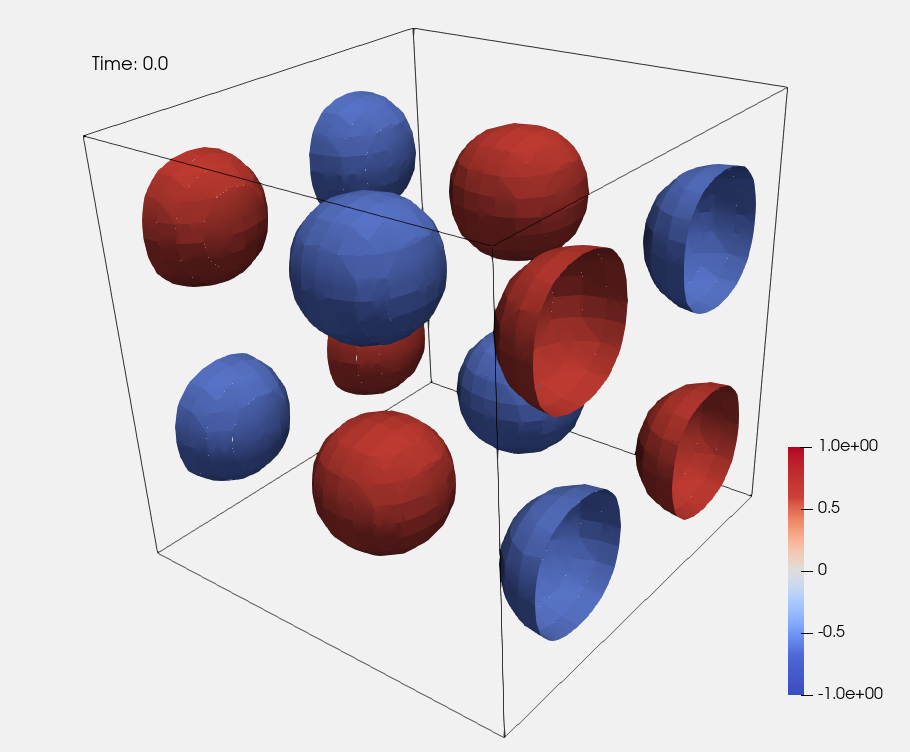
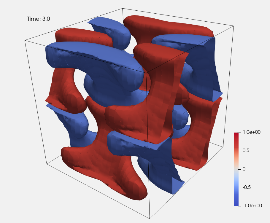
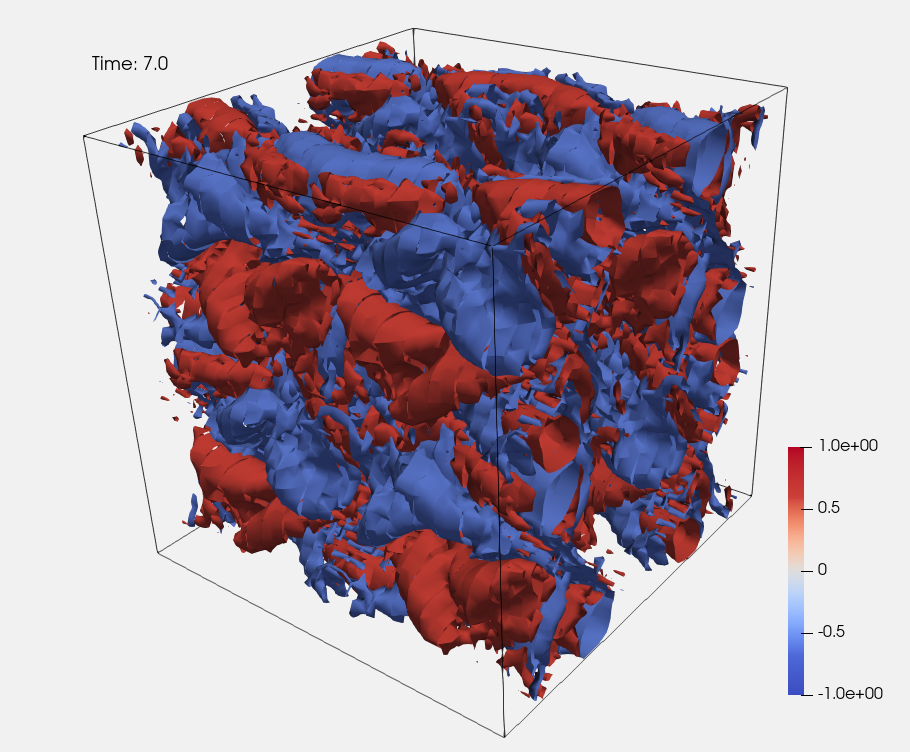
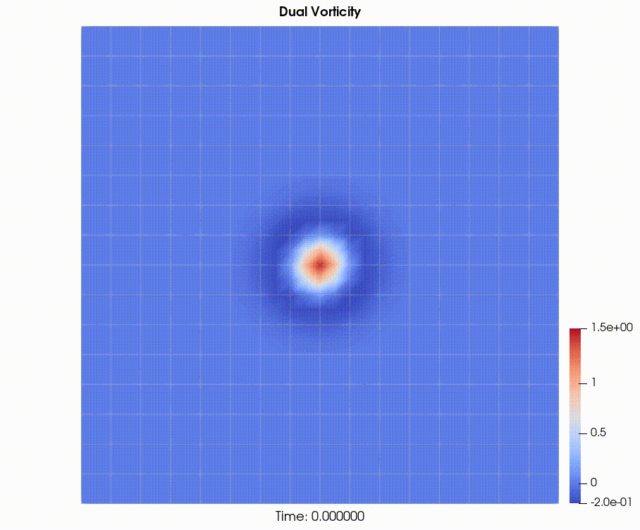
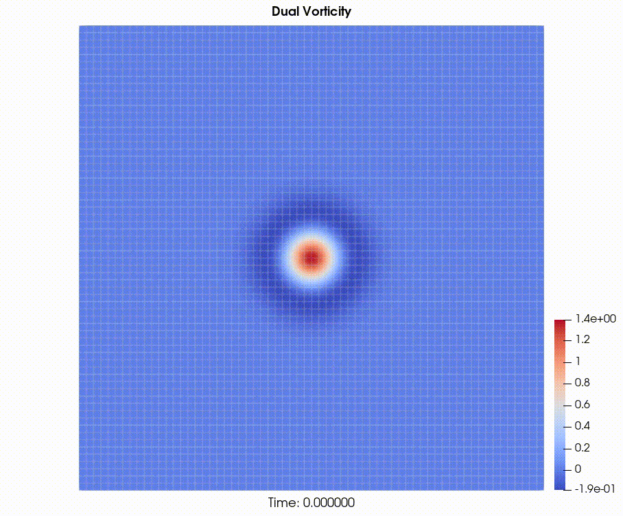
The Taylor-Green Vortex problem is a classic benchmark problem in fluid dynamics for 2D and 3D, where in the former it has an exact analytical solution. The spatial domain is given by [math] [\pi,\pi]^n [/math]. The initial condition starts with a number of developed vortices in the flow. If viscosity is zero, the numerical solution should ideally not distort the vortices and the kinetic energy should remain constant for all time. For a viscous flow, the vortices should disappear monotonically as the kinetic energy dissipates as demonstrated in the 2D experiment below where the evolution of the dual vorticity field is shown in addition to the Kinetic Energy and Enstrophy evolution with time compared with the exact solution.
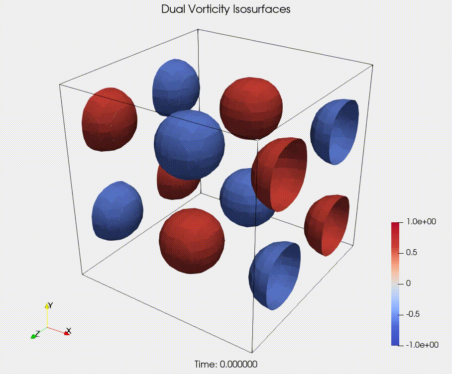
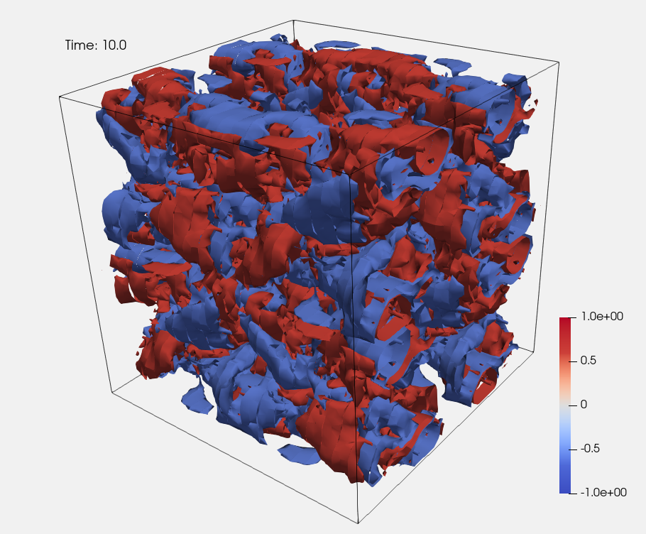
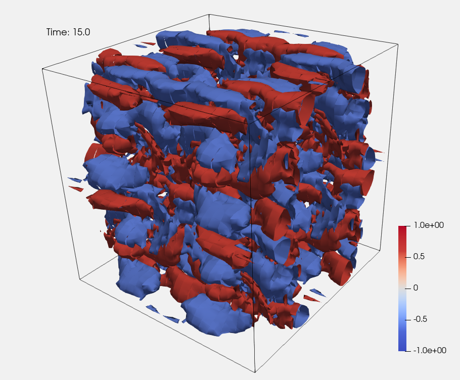
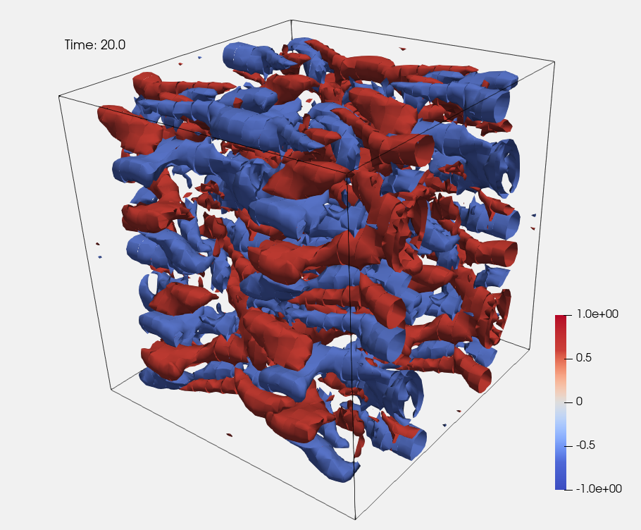
In the case of 3D, the viscosity effects lead to a breaking and stretching of the vortex structures. In the Animations and Snapshots below, we show the evolution of the dual-vorticity x-component for [math] t \in \{0,20\} \text{sec} [/math] for a coarse mesh 24p2 and a fine mesh 24p3.
In the plots below we compare the dual-field solver with the DNS results of Brachet et al. 1983 [2] and the compact finite difference solver of Caban & Tyliszczak 2022 for a [math] 256^3 [/math] mesh [3].

Vortex Advection problem
In this benchmark problem, the flow is solved in a periodic domain spanning the region [math] [-10,10]^2 [/math] with an initial vortex centered at (0,0). Since inviscid flow is assumed, the vortex should be advected without any deformation or decay. Thus, the effect of numerical/artificial dissipation of the dual-field method can be tested with this problem. A comparison between a coarse mesh (16p2) and a fine mesh (64p2) is shown below.
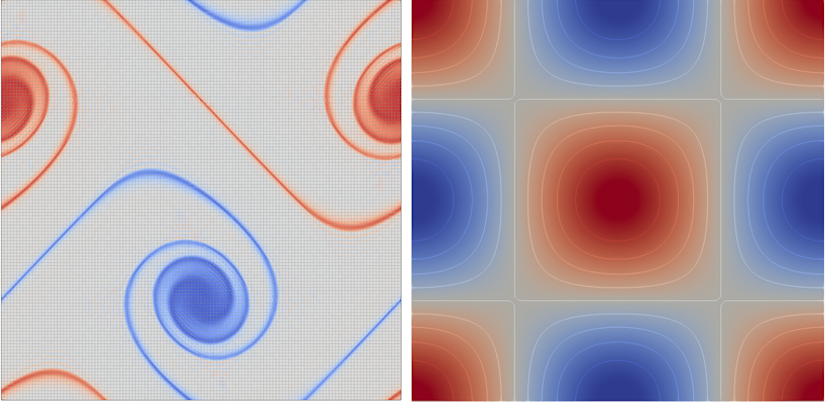
Inviscid Shear Layer problem
This benchmark test case, also known as the double jet problem, is widely used to verify the accuracy of discretization schemes in a range of the small-scale phenomena (large wave numbers) generated when the flow evolves in time. In a periodic box of [math] [-\pi,\pi]^2 [/math], the initial velocity field at [math] t=0 [/math] forms two parallel shear layers, one with positive vorticity and the other with negative. The small perturbation in the vertical component grows with time and leads to a roll-up of the shear layers and formation of the vortex cores. As the time passes, the shear layers between the vortices are stretched and become thinner. Consequently, small flow structures appear of which a proper representation requires a highly accurate discretization method [3]. Below we show the resutls of the dual-field scheme for 16p2, 64p2 and 128p2.

16p2 Animation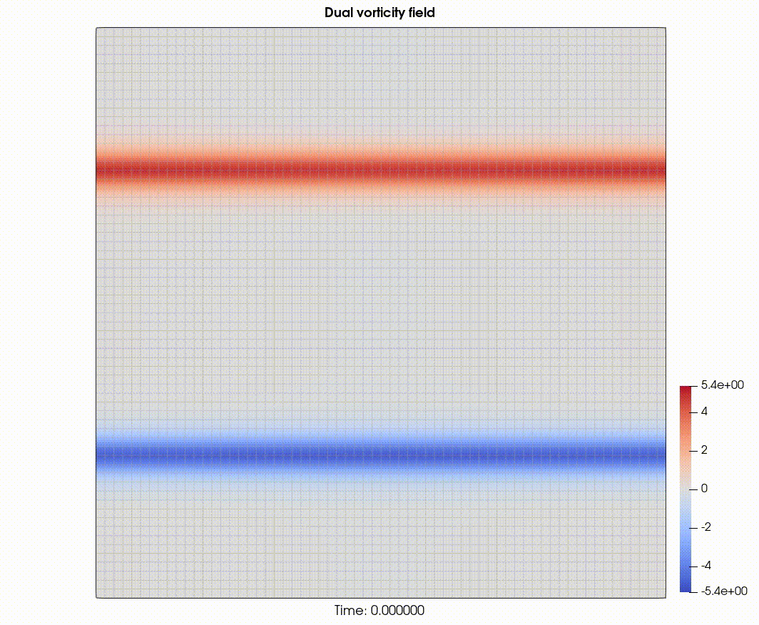

References
[1] Zhang, Y., Palha, A., Gerritsma, M., & Rebholz, L. G. (2022). A mass-, kinetic energy-and helicity-conserving mimetic dual-field discretization for three-dimensional incompressible Navier-Stokes equations, part I: Periodic domains. Journal of Computational Physics, 451, 110868.
[2] Brachet, M.E., Meiron, D.I., Orszag, S.A., Nickel, B.G., Morf, R.H. and Frisch, U., Small-scale structure of the Taylor–Green vortex. J. Fluid Mech. 1983, 130, 441–452.
[3] Caban, L., & Tyliszczak, A. (2022). High-order compact difference schemes on wide computational stencils with a spectral-like accuracy. Computers & Mathematics with Applications, 108, 123-140.